Querying the structure pool for the Cs-Te binary system¶

This example is reproducing the steps to create the initial structure pool for the high-throughput calculations published here:doi:10.1063/5.0082710.

As an initial data pool of crystal structures we use the Materials Project (MP) database and the Open Quantum Materials database (OQMD) that can be readily interfaced using the StructureImporter class of the library:

[1]:

from aim2dat.strct import StructureImporter

strct_imp = StructureImporter()

Querying crystals from Materials Project and Open Quantum Materials Database¶

The first argument for the queries consists of the chemical compositions specified via the string 'Cs-Te'.

As for the MP database we query the initial structures (specified via the keyword structure_type) since these structures still have all symmetries. Additionally, an individual API key has to be passed to the function which can be requested at the MP webpage.

Update: The original interface to materials project via the pymatgen library is depreciated and will be removed soon. It is advised to use the open-api by setting the keyword argument use_openapi to True.

[2]:

import os

strct_imp.import_from_mp(
    "Cs-Te", "NiQf1wbOAEUJHo8H", structure_type="initial", use_openapi=False
)

/opt/hostedtoolcache/Python/3.10.15/x64/lib/python3.10/site-packages/pymatgen/ext/matproj_legacy.py:164: UserWarning: You are using the legacy MPRester. This version of the MPRester will no longer be updated. To access the latest data with the new MPRester, obtain a new API key from https://materialsproject.org/api and consult the docs at https://docs.materialsproject.org/ for more information.
  warnings.warn(

connected with Materials Project Version 2020_09_08.

/opt/hostedtoolcache/Python/3.10.15/x64/lib/python3.10/site-packages/pymatgen/ext/matproj_legacy.py:164: UserWarning: You are using the legacy MPRester. This version of the MPRester will no longer be updated. To access the latest data with the new MPRester, obtain a new API key from https://materialsproject.org/api and consult the docs at https://docs.materialsproject.org/ for more information.
  warnings.warn(

connected with Materials Project Version 2020_09_08.

/opt/hostedtoolcache/Python/3.10.15/x64/lib/python3.10/site-packages/pymatgen/ext/matproj_legacy.py:164: UserWarning: You are using the legacy MPRester. This version of the MPRester will no longer be updated. To access the latest data with the new MPRester, obtain a new API key from https://materialsproject.org/api and consult the docs at https://docs.materialsproject.org/ for more information.
  warnings.warn(

connected with Materials Project Version 2020_09_08.

[2]:

<aim2dat.strct.structure_collection.StructureCollection at 0x7f68ca8f1810>

[3]:

strct_imp.import_from_oqmd("Cs-Te", query_limit=1000)

[3]:

<aim2dat.strct.structure_collection.StructureCollection at 0x7f68ca569e70>

The downloaded crystals are stored in a StructureCollection object which can be accessed via the structures property. We can check the number of imported structures via len or by printing the object:

[4]:

len(strct_imp.structures)

[4]:

[5]:

print(strct_imp)

----------------------------------------------------------------------
------------------------ Structure Collection ------------------------
----------------------------------------------------------------------

                          Imported from: mp
   - Number of structures: 32
   - Elements: Cs-Te

                         Imported from: oqmd
   - Number of structures: 124
   - Elements: Cs-Te

----------------------------------------------------------------------

                     Chemical element constraints
   Neglecting elemental structures: False

                     Chemical formula constraints
   Not set.

                        Attribute constraints
   Not set.

----------------------------------------------------------------------

Since we have been querying data from two different databases we might also want to check whether there are crystals shared by both databases. In this case we use the F-fingerprint (doi:10.1063/1.3079326) to identify duplicate structures. The function to indentify duplicate structures is implemented in the StructureOperations class.

We can simply pass the StructureCollection](aiida_scripts.structure_analysis.StructureCollection) object from the StructureImporter to the StructureOperations object upon initialization:

[6]:

from aim2dat.strct import StructureOperations

strct_op = StructureOperations(structures=strct_imp.structures)
strct_op.n_procs = 2
strct_op.cunksize = 500
strct_op.verbose = False

We use the find_duplicates_via_ffingerprint function to identify duplicate crystals, the function returns the labels of duplicate pairs and removes the first member of the pair from the StructureCollection object if remove_structures is set to True:

[7]:

strct_op.find_duplicates_via_ffingerprint(
    remove_structures=True,
    threshold=0.001,
    r_max=15.0,
    delta_bin=0.005,
    sigma=10.0
)

[7]:

[('OQMD_676192', 'mp_mp-1055940'),
 ('OQMD_676503', 'mp_mp-1055940'),
 ('OQMD_676504', 'mp_mp-1055940'),
 ('OQMD_621965', 'OQMD_620946'),
 ('OQMD_677954', 'OQMD_676288'),
 ('OQMD_1280348', 'OQMD_1215022'),
 ('OQMD_690486', 'OQMD_676083'),
 ('OQMD_675565', 'OQMD_675564'),
 ('OQMD_676082', 'OQMD_686178')]

Once again we can check the final number of structures:

[8]:

len(strct_op.structures)

[8]:

Analysing the initial dataset¶

Having the duplicate structures removed we can split the dataset based on the crystal’s source database:

[9]:

structures_mp = strct_op.structures[:32]
structures_oqmd = strct_op.structures[32:]

We can get a better overview of on the crystals by exporting the data into a pandas dataframe for better visualization:

[10]:

df_mp = structures_mp.create_pandas_df(
    exclude_columns=["functional", "icsd_ids", "magnetic_moment", "direct_band_gap"]
)
df_mp

[10]:

	label	el_conc_Cs	el_conc_Te	nr_atoms	nr_atoms_Cs	nr_atoms_Te	source	source_id	space_group	formation_energy (eV/atom)	stability (eV/atom)
0	mp_mp-1012110	1.000000	0.000000	4	4	0	MP_2020_09_08	mp-1012110	57	0.046335	0.046335
1	mp_mp-949029	1.000000	0.000000	8	8	0	MP_2020_09_08	mp-949029	223	0.046690	0.046690
2	mp_mp-1055940	1.000000	0.000000	1	1	0	MP_2020_09_08	mp-1055940	225	0.041371	0.041371
3	mp_mp-573579	1.000000	0.000000	8	8	0	MP_2020_09_08	mp-573579	64	0.053976	0.053976
4	mp_mp-639727	1.000000	0.000000	4	4	0	MP_2020_09_08	mp-639727	194	0.026213	0.026213
5	mp_mp-1183897	1.000000	0.000000	20	20	0	MP_2020_09_08	mp-1183897	213	0.038677	0.038677
6	mp_mp-672241	1.000000	0.000000	8	8	0	MP_2020_09_08	mp-672241	135	0.065470	0.065470
7	mp_mp-1	1.000000	0.000000	1	1	0	MP_2020_09_08	mp-1	229	0.038770	0.038770
8	mp_mp-11832	1.000000	0.000000	2	2	0	MP_2020_09_08	mp-11832	194	0.035109	0.035109
9	mp_mp-1096915	1.000000	0.000000	1	1	0	MP_2020_09_08	mp-1096915	12	0.042218	0.042218
10	mp_mp-1007976	1.000000	0.000000	4	4	0	MP_2020_09_08	mp-1007976	62	0.054917	0.054917
11	mp_mp-1184151	1.000000	0.000000	29	29	0	MP_2020_09_08	mp-1184151	217	0.000000	0.000000
12	mp_mp-1183694	1.000000	0.000000	1	1	0	MP_2020_09_08	mp-1183694	139	0.037375	0.037375
13	mp_mp-3	1.000000	0.000000	2	2	0	MP_2020_09_08	mp-3	141	0.097650	0.097650
14	mp_mp-1178932	0.000000	1.000000	1	0	1	MP_2020_09_08	mp-1178932	166	0.054101	0.054101
15	mp_mp-9924	0.000000	1.000000	1	0	1	MP_2020_09_08	mp-9924	65	0.127402	0.127402
16	mp_mp-1178952	0.000000	1.000000	4	0	4	MP_2020_09_08	mp-1178952	26	0.049131	0.049131
17	mp_mp-1064307	0.000000	1.000000	4	0	4	MP_2020_09_08	mp-1064307	18	0.122781	0.122781
18	mp_mp-19	0.000000	1.000000	3	0	3	MP_2020_09_08	mp-19	152	0.000000	0.000000
19	mp_mp-567313	0.000000	1.000000	3	0	3	MP_2020_09_08	mp-567313	154	0.000024	0.000024
20	mp_mp-570459	0.000000	1.000000	3	0	3	MP_2020_09_08	mp-570459	12	0.043651	0.043651
21	mp_mp-105	0.000000	1.000000	4	0	4	MP_2020_09_08	mp-105	51	0.047063	0.047063
22	mp_mp-10654	0.000000	1.000000	1	0	1	MP_2020_09_08	mp-10654	221	0.046556	0.046556
23	mp_mp-8361	0.500000	0.500000	8	4	4	MP_2020_09_08	mp-8361	55	-0.847515	0.000000
24	mp_mp-1178386	0.200000	0.800000	20	4	16	MP_2020_09_08	mp-1178386	14	-0.391677	0.000000
25	mp_mp-620471	0.120000	0.880000	25	3	22	MP_2020_09_08	mp-620471	1	-0.212136	0.022870
26	mp_mp-573763	0.666667	0.333333	12	8	4	MP_2020_09_08	mp-573763	62	-0.991598	0.000000
27	mp_mp-505464	0.133333	0.866667	60	8	52	MP_2020_09_08	mp-505464	57	-0.257485	0.003632
28	mp_mp-1205022	0.125000	0.875000	128	16	112	MP_2020_09_08	mp-1205022	130	-0.214743	0.030055
29	mp_mp-505634	0.400000	0.600000	10	4	6	MP_2020_09_08	mp-505634	36	-0.742686	0.000000
30	mp_mp-1188281	0.625000	0.375000	16	10	6	MP_2020_09_08	mp-1188281	87	-0.955132	0.000445
31	mp_mp-1191593	0.120000	0.880000	25	3	22	MP_2020_09_08	mp-1191593	87	-0.204884	0.030122

[11]:

df_oqmd = structures_oqmd.create_pandas_df(
    exclude_columns=["functional", "icsd_ids", "magnetic_moment", "direct_band_gap"]
)

The dataset can be analyzed in more detail using the PhasePlot object from the plot sub-package of the library:

[12]:

from aim2dat.plots import PhasePlot

Here we use the matplotlib-library to create the plots, interactive plots can also be generated by changing the backend to "plotly":

[13]:

phase_diagram = PhasePlot()
phase_diagram.ratio = (9, 4.5)
phase_diagram.show_crystal_system = True
phase_diagram.show_legend = True
phase_diagram.legend_bbox_to_anchor = (1.35, 1.0)
phase_diagram.backend = "matplotlib"

Chemical composition and formation energies can be readily parsed from the pandas data frames:

[14]:

phase_diagram.import_from_pandas_df("MP", df_mp)
phase_diagram.import_from_pandas_df("OQMD", df_oqmd)

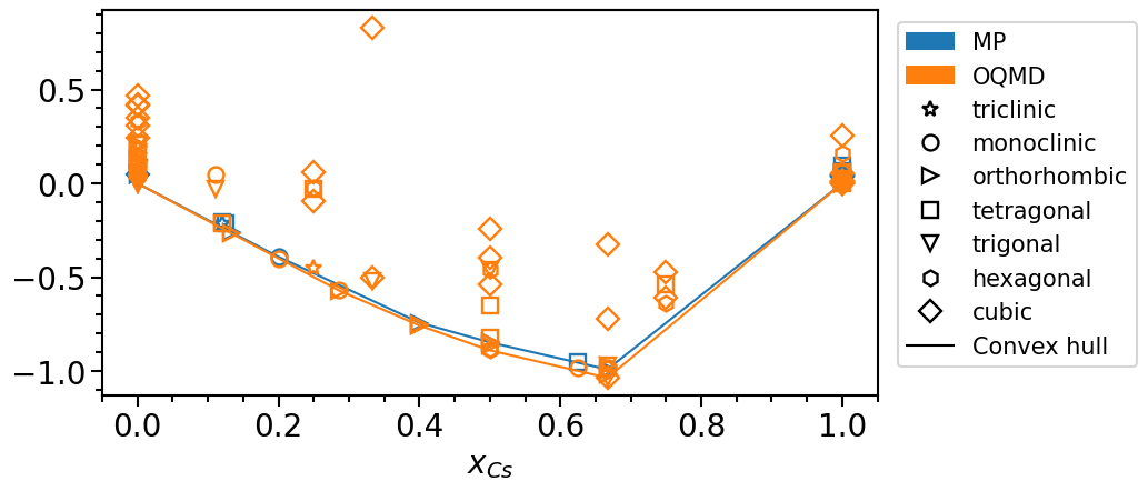
[15]:

phase_diagram.plot_type = "scatter"
phase_diagram.plot_property = "formation_energy"
phase_diagram.plot(["MP", "OQMD"])

[15]:

../_images/examples_strct-odb_interfaces_25_0.png

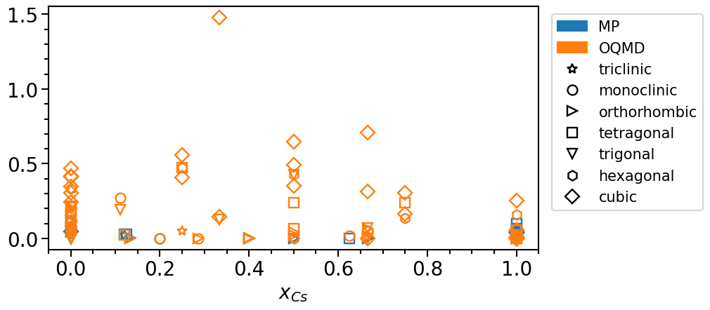
The stability is defined as the vertical distance of a phase with respect to the convex hull:

[16]:

phase_diagram.plot_property = "stability"
phase_diagram.show_convex_hull = False
phase_diagram.plot(["MP", "OQMD"])

[16]:

../_images/examples_strct-odb_interfaces_27_0.png

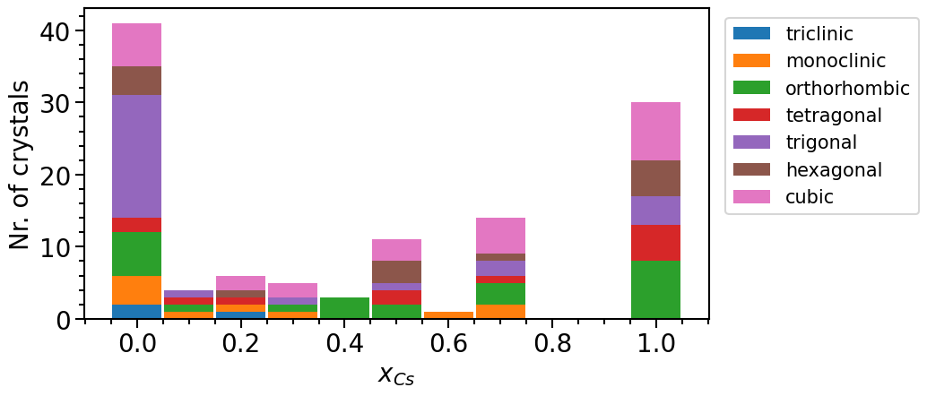
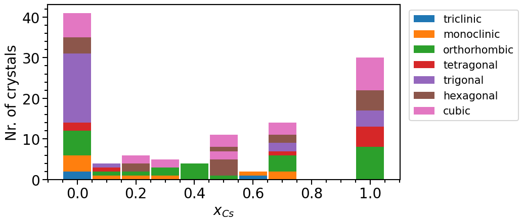
To analyze the distribution of the phases in their chemical configuration space we can plot a histogram of the total number of phases per concentration interval and crystal system:

[17]:

phase_diagram.plot_type = "numbers"
phase_diagram.y_label = "Nr. of crystals"
phase_diagram.plot(["MP", "OQMD"])

[17]:

../_images/examples_strct-odb_interfaces_29_0.png

Exploiting chemical similarity to increase the structure pool¶

From the last plot it is noticeable that more than two thirds of the structures actually represent elemental phases. This imbalance is due to the fact that most structures in online databases have been determined experimentally. Thus, we often find that the chemical space (in this case the mixed phases) relevant is under-represented in the dataset because it is easier to experimentally analyze “simple” compounds.

One way to counteract this trend is to make use of the chemical similarity of cations or anions and also query structures containing of ions having the same oxidation state as the target system. The ions can then be replaced in a second step, thus obtaining a larger variety of structures. To do so, we import new structures once again. However, this time we exclude elemental phases straight-away by setting the corresponding constraint:

[18]:

strct_imp = StructureImporter()
strct_imp.neglect_elemental_structures = True

[19]:

strct_imp.import_from_mp(
    ["K-Te", "Rb-Te", "K-Se", "Rb-Se", "Cs-Se", "K-Po", "Rb-Po", "Cs-Po"],
    "NiQf1wbOAEUJHo8H",
    structure_type="initial",
    use_openapi=False,
)

/opt/hostedtoolcache/Python/3.10.15/x64/lib/python3.10/site-packages/pymatgen/ext/matproj_legacy.py:164: UserWarning: You are using the legacy MPRester. This version of the MPRester will no longer be updated. To access the latest data with the new MPRester, obtain a new API key from https://materialsproject.org/api and consult the docs at https://docs.materialsproject.org/ for more information.
  warnings.warn(

connected with Materials Project Version 2020_09_08.

/opt/hostedtoolcache/Python/3.10.15/x64/lib/python3.10/site-packages/pymatgen/ext/matproj_legacy.py:164: UserWarning: You are using the legacy MPRester. This version of the MPRester will no longer be updated. To access the latest data with the new MPRester, obtain a new API key from https://materialsproject.org/api and consult the docs at https://docs.materialsproject.org/ for more information.
  warnings.warn(

connected with Materials Project Version 2020_09_08.

/opt/hostedtoolcache/Python/3.10.15/x64/lib/python3.10/site-packages/pymatgen/ext/matproj_legacy.py:164: UserWarning: You are using the legacy MPRester. This version of the MPRester will no longer be updated. To access the latest data with the new MPRester, obtain a new API key from https://materialsproject.org/api and consult the docs at https://docs.materialsproject.org/ for more information.
  warnings.warn(

connected with Materials Project Version 2020_09_08.

/opt/hostedtoolcache/Python/3.10.15/x64/lib/python3.10/site-packages/pymatgen/ext/matproj_legacy.py:164: UserWarning: You are using the legacy MPRester. This version of the MPRester will no longer be updated. To access the latest data with the new MPRester, obtain a new API key from https://materialsproject.org/api and consult the docs at https://docs.materialsproject.org/ for more information.
  warnings.warn(

connected with Materials Project Version 2020_09_08.

/opt/hostedtoolcache/Python/3.10.15/x64/lib/python3.10/site-packages/pymatgen/ext/matproj_legacy.py:164: UserWarning: You are using the legacy MPRester. This version of the MPRester will no longer be updated. To access the latest data with the new MPRester, obtain a new API key from https://materialsproject.org/api and consult the docs at https://docs.materialsproject.org/ for more information.
  warnings.warn(

connected with Materials Project Version 2020_09_08.

/opt/hostedtoolcache/Python/3.10.15/x64/lib/python3.10/site-packages/pymatgen/ext/matproj_legacy.py:164: UserWarning: You are using the legacy MPRester. This version of the MPRester will no longer be updated. To access the latest data with the new MPRester, obtain a new API key from https://materialsproject.org/api and consult the docs at https://docs.materialsproject.org/ for more information.
  warnings.warn(

connected with Materials Project Version 2020_09_08.

/opt/hostedtoolcache/Python/3.10.15/x64/lib/python3.10/site-packages/pymatgen/ext/matproj_legacy.py:164: UserWarning: You are using the legacy MPRester. This version of the MPRester will no longer be updated. To access the latest data with the new MPRester, obtain a new API key from https://materialsproject.org/api and consult the docs at https://docs.materialsproject.org/ for more information.
  warnings.warn(

connected with Materials Project Version 2020_09_08.

/opt/hostedtoolcache/Python/3.10.15/x64/lib/python3.10/site-packages/pymatgen/ext/matproj_legacy.py:164: UserWarning: You are using the legacy MPRester. This version of the MPRester will no longer be updated. To access the latest data with the new MPRester, obtain a new API key from https://materialsproject.org/api and consult the docs at https://docs.materialsproject.org/ for more information.
  warnings.warn(

connected with Materials Project Version 2020_09_08.

[19]:

<aim2dat.strct.structure_collection.StructureCollection at 0x7f68e36a6a10>

[20]:

strct_imp.import_from_oqmd(
    ["K-Te", "Rb-Te", "K-Se", "Rb-Se", "Cs-Se", "K-Po", "Rb-Po", "Cs-Po"], query_limit=1000
)

[20]:

<aim2dat.strct.structure_collection.StructureCollection at 0x7f68c78ea0b0>

Now we can substitute the elements in StructureOperations object accordingly:

[21]:

strct_op.structures = strct_imp.structures
structures_subst = strct_op[strct_op.structures.labels].substitute_elements(
    [("K", "Cs"), ("Rb", "Cs"), ("Se", "Te"), ("Po", "Te")],
    change_label=True,
)

Since we have now probably have quite a few duplicate structures we will try to remove them. This time, however, we use a less strict method to filter out structures that are likely to be duplicates of others using merely the composition and the space group as criteria.

Note: In order to reduce the run time, we only take the first 50 crystals for this example.

We can choose to restrict the method merely on the newly imported structures where we substituted the elements by using the confined keyword, thus keeping all the previous phases in our dataset and applying the tight constraint only on the newly created phases:

[22]:

strct_op.structures = structures_mp + structures_oqmd + structures_subst[:50]
strct_op.find_duplicates_via_comp_sym(remove_structures=True, confined=(133, 133 + 50))

spglib: No point group was found (line 405, /project/src/pointgroup.c).
spglib: Attempt 0 tolerance = 5.000000e-03 failed(line 800, /project/src/spacegroup.c).
spglib: No point group was found (line 405, /project/src/pointgroup.c).
spglib: Attempt 1 tolerance = 4.750000e-03 failed(line 800, /project/src/spacegroup.c).
spglib: No point group was found (line 405, /project/src/pointgroup.c).
spglib: Attempt 2 tolerance = 4.512500e-03 failed(line 800, /project/src/spacegroup.c).
spglib: No point group was found (line 405, /project/src/pointgroup.c).
spglib: Attempt 3 tolerance = 4.286875e-03 failed(line 800, /project/src/spacegroup.c).
spglib: No point group was found (line 405, /project/src/pointgroup.c).
spglib: Attempt 4 tolerance = 4.072531e-03 failed(line 800, /project/src/spacegroup.c).
spglib: No point group was found (line 405, /project/src/pointgroup.c).
spglib: Attempt 5 tolerance = 3.868905e-03 failed(line 800, /project/src/spacegroup.c).
spglib: No point group was found (line 405, /project/src/pointgroup.c).
spglib: Attempt 6 tolerance = 3.675459e-03 failed(line 800, /project/src/spacegroup.c).
spglib: No point group was found (line 405, /project/src/pointgroup.c).
spglib: Attempt 0 tolerance = 5.000000e-03 failed(line 800, /project/src/spacegroup.c).
spglib: No point group was found (line 405, /project/src/pointgroup.c).
spglib: Attempt 1 tolerance = 4.750000e-03 failed(line 800, /project/src/spacegroup.c).
spglib: No point group was found (line 405, /project/src/pointgroup.c).
spglib: Attempt 2 tolerance = 4.512500e-03 failed(line 800, /project/src/spacegroup.c).
spglib: No point group was found (line 405, /project/src/pointgroup.c).
spglib: Attempt 3 tolerance = 4.286875e-03 failed(line 800, /project/src/spacegroup.c).
spglib: No point group was found (line 405, /project/src/pointgroup.c).
spglib: Attempt 4 tolerance = 4.072531e-03 failed(line 800, /project/src/spacegroup.c).
spglib: No point group was found (line 405, /project/src/pointgroup.c).
spglib: Attempt 5 tolerance = 3.868905e-03 failed(line 800, /project/src/spacegroup.c).
spglib: No point group was found (line 405, /project/src/pointgroup.c).
spglib: Attempt 6 tolerance = 3.675459e-03 failed(line 800, /project/src/spacegroup.c).

spglib: No point group was found (line 405, /project/src/pointgroup.c).
spglib: Attempt 0 tolerance = 5.000000e-03 failed(line 800, /project/src/spacegroup.c).
spglib: No point group was found (line 405, /project/src/pointgroup.c).
spglib: Attempt 1 tolerance = 4.750000e-03 failed(line 800, /project/src/spacegroup.c).
spglib: No point group was found (line 405, /project/src/pointgroup.c).
spglib: Attempt 2 tolerance = 4.512500e-03 failed(line 800, /project/src/spacegroup.c).
spglib: No point group was found (line 405, /project/src/pointgroup.c).
spglib: Attempt 3 tolerance = 4.286875e-03 failed(line 800, /project/src/spacegroup.c).
spglib: No point group was found (line 405, /project/src/pointgroup.c).
spglib: Attempt 4 tolerance = 4.072531e-03 failed(line 800, /project/src/spacegroup.c).
spglib: No point group was found (line 405, /project/src/pointgroup.c).
spglib: Attempt 5 tolerance = 3.868905e-03 failed(line 800, /project/src/spacegroup.c).
spglib: No point group was found (line 405, /project/src/pointgroup.c).
spglib: Attempt 6 tolerance = 3.675459e-03 failed(line 800, /project/src/spacegroup.c).
spglib: No point group was found (line 405, /project/src/pointgroup.c).
spglib: Attempt 7 tolerance = 3.491686e-03 failed(line 800, /project/src/spacegroup.c).
spglib: No point group was found (line 405, /project/src/pointgroup.c).
spglib: Attempt 8 tolerance = 3.317102e-03 failed(line 800, /project/src/spacegroup.c).
spglib: No point group was found (line 405, /project/src/pointgroup.c).
spglib: Attempt 9 tolerance = 3.151247e-03 failed(line 800, /project/src/spacegroup.c).
spglib: No point group was found (line 405, /project/src/pointgroup.c).
spglib: Attempt 10 tolerance = 2.993685e-03 failed(line 800, /project/src/spacegroup.c).
spglib: No point group was found (line 405, /project/src/pointgroup.c).
spglib: Attempt 0 tolerance = 5.000000e-03 failed(line 800, /project/src/spacegroup.c).
spglib: No point group was found (line 405, /project/src/pointgroup.c).
spglib: Attempt 1 tolerance = 4.750000e-03 failed(line 800, /project/src/spacegroup.c).
spglib: No point group was found (line 405, /project/src/pointgroup.c).
spglib: Attempt 2 tolerance = 4.512500e-03 failed(line 800, /project/src/spacegroup.c).
spglib: No point group was found (line 405, /project/src/pointgroup.c).
spglib: Attempt 3 tolerance = 4.286875e-03 failed(line 800, /project/src/spacegroup.c).
spglib: No point group was found (line 405, /project/src/pointgroup.c).
spglib: Attempt 4 tolerance = 4.072531e-03 failed(line 800, /project/src/spacegroup.c).
spglib: No point group was found (line 405, /project/src/pointgroup.c).
spglib: Attempt 5 tolerance = 3.868905e-03 failed(line 800, /project/src/spacegroup.c).
spglib: No point group was found (line 405, /project/src/pointgroup.c).
spglib: Attempt 6 tolerance = 3.675459e-03 failed(line 800, /project/src/spacegroup.c).
spglib: No point group was found (line 405, /project/src/pointgroup.c).
spglib: Attempt 7 tolerance = 3.491686e-03 failed(line 800, /project/src/spacegroup.c).
spglib: No point group was found (line 405, /project/src/pointgroup.c).
spglib: Attempt 8 tolerance = 3.317102e-03 failed(line 800, /project/src/spacegroup.c).
spglib: No point group was found (line 405, /project/src/pointgroup.c).
spglib: Attempt 9 tolerance = 3.151247e-03 failed(line 800, /project/src/spacegroup.c).
spglib: No point group was found (line 405, /project/src/pointgroup.c).
spglib: Attempt 10 tolerance = 2.993685e-03 failed(line 800, /project/src/spacegroup.c).

[22]:

[('mp_mp-8360_subst-RbCs', 'mp_mp-8361'),
 ('mp_mp-568745_subst-RbCs', 'mp_mp-573763'),
 ('mp_mp-1397_subst-RbCs', 'mp_mp-573763'),
 ('mp_mp-1011696_subst-SeTe', 'mp_mp-573763'),
 ('OQMD_647134', 'mp_mp-505634'),
 ('mp_mp-7670_subst-KCs-SeTe', 'mp_mp-505634'),
 ('mp_mp-7447_subst-RbCs-SeTe', 'mp_mp-505634'),
 ('mp_mp-644_subst-KCs', 'mp_mp-1188281'),
 ('mp_mp-755633_subst-KCs-SeTe', 'mp_mp-1188281'),
 ('mp_mp-1009489_subst-RbCs', 'OQMD_1104417'),
 ('mp_mp-1059621_subst-KCs-SeTe', 'OQMD_1104417'),
 ('mp_mp-1061530_subst-RbCs-SeTe', 'OQMD_1104417'),
 ('mp_mp-1009491_subst-RbCs', 'OQMD_1222159'),
 ('OQMD_1593007', 'OQMD_1239241'),
 ('mp_mp-1747_subst-KCs', 'OQMD_1343671'),
 ('mp_mp-441_subst-RbCs', 'OQMD_1343671'),
 ('mp_mp-8426_subst-KCs-SeTe', 'OQMD_1343671'),
 ('mp_mp-11327_subst-RbCs-SeTe', 'OQMD_1343671'),
 ('mp_mp-1011695_subst-SeTe', 'OQMD_1343671'),
 ('mp_mp-31002_subst-RbCs', 'OQMD_1800027'),
 ('mp_mp-2095_subst-RbCs', 'mp_mp-7289_subst-KCs'),
 ('mp_mp-9064_subst-RbCs', 'mp_mp-1554_subst-KCs'),
 ('mp_mp-9268_subst-KCs-SeTe', 'mp_mp-1554_subst-KCs'),
 ('mp_mp-9063_subst-RbCs-SeTe', 'mp_mp-1554_subst-KCs'),
 ('mp_mp-1080254_subst-SeTe', 'mp_mp-383_subst-RbCs'),
 ('mp_mp-1180659_subst-KCs-SeTe', 'mp_mp-1080121_subst-KCs-SeTe'),
 ('mp_mp-620372_subst-RbCs-SeTe', 'mp_mp-18609_subst-KCs-SeTe'),
 ('mp_mp-18609_subst-KCs-SeTe', 'mp_mp-541055_subst-SeTe')]

And now we can add the new structures to our plot object:

[23]:

subst_structures = strct_op.structures[133:]
df_subst = subst_structures.create_pandas_df(
    exclude_columns=["functional", "icsd_ids", "magnetic_moment", "direct_band_gap"]
)
df_subst
phase_diagram.import_from_pandas_df("subst. structures", df_subst)
phase_diagram.plot(["MP", "OQMD", "subst. structures"])

[23]:

../_images/examples_strct-odb_interfaces_39_0.png

We can clearly see that the number of mixed phases is larger in the new data pool.