Creating a discretized grid to analyse functions¶

Create a discretized axis¶

The DiscretizedAxis object allows to discretize a given range e.g. an energy or DOS range. At the moment, uniformly and normally distributed discretizations are implemented. The method can be chosen via discretization_method. Either a string specifying the implemented methods or a custom function are allowed.

The DiscretizedAxis expects the axis_type argument, this can be either “x” or “y”. The other attributes can be set afterwards. The axis_type specifies the shape of the internal numpy array that stores the values of the axis.

Create Two axis, both of axis_type x but with different ranges and discretization types. The normal discretization expects a mean and standard deviation. In case of the uniform distribution, no further keywords are needed and the step size is specified via min_step.

Further arguments of the class are:

• min, max: Specify the minimum and maximum value of the axis

• max_num_steps: Specifies the maximum step size for the gaussian distributed discretization which is max_num_steps multiplied with min_step.

[1]:

from aim2dat.fct import DiscretizedAxis

axis = DiscretizedAxis(axis_type="x", max=0.49, min=0, min_step=0.01)
axis.discretization_method = "gaussian"
axis.discretize_axis(mu=1, sigma=2)

axis2 = DiscretizedAxis(axis_type="x", max=1, min=0, min_step=0.02)
axis2.discretization_method = "uniform"
axis2.discretize_axis()

[1]:

DiscretizedAxis
        axis_type: x
        max: 1
        min: 0
        min_step: 0.02
        max_num_steps: 5
        precision: 6
        discretization_method: _uniform_discretization

<aim2dat.fct.discretization.DiscretizedAxis object at 0x7fb9944dee30>

We can now check that the axis is uniformly distributed.

[2]:

axis.axis

[2]:

array([[0.  , 0.01, 0.03, 0.05, 0.06, 0.07, 0.08, 0.09, 0.1 , 0.11, 0.12,
        0.13, 0.14, 0.15, 0.16, 0.17, 0.18, 0.19, 0.2 , 0.21, 0.22, 0.23,
        0.24, 0.25, 0.26, 0.27, 0.28, 0.29, 0.3 , 0.31, 0.32, 0.33, 0.34,
        0.35, 0.36, 0.37, 0.38, 0.39, 0.4 , 0.41, 0.42, 0.43, 0.44, 0.45,
        0.46, 0.47, 0.48, 0.49]])

Normally distributed.

[3]:

axis2.axis

[3]:

array([[0.  , 0.02, 0.04, 0.06, 0.08, 0.1 , 0.12, 0.14, 0.16, 0.18, 0.2 ,
        0.22, 0.24, 0.26, 0.28, 0.3 , 0.32, 0.34, 0.36, 0.38, 0.4 , 0.42,
        0.44, 0.46, 0.48, 0.5 , 0.52, 0.54, 0.56, 0.58, 0.6 , 0.62, 0.64,
        0.66, 0.68, 0.7 , 0.72, 0.74, 0.76, 0.78, 0.8 , 0.82, 0.84, 0.86,
        0.88, 0.9 , 0.92, 0.94, 0.96, 0.98, 1.  ]])

Merge two objects with the same axis_type¶

The addition of two DiscretizedAxis objects leads to a merge of the two axis ranges. The axis of the first summand is kept. In case the second summand covers a range that is not covered by the first one, the part will be merged. Before the ranges are merged, the last point of the first summand and the first point of the merged range are aligned.

[4]:

axis3 = axis + axis2

The merge is performed at 0.49. The values of the axis2 are shifted as mentioned before.

[5]:

axis3.axis

[5]:

array([[0.  , 0.01, 0.03, 0.05, 0.06, 0.07, 0.08, 0.09, 0.1 , 0.11, 0.12,
        0.13, 0.14, 0.15, 0.16, 0.17, 0.18, 0.19, 0.2 , 0.21, 0.22, 0.23,
        0.24, 0.25, 0.26, 0.27, 0.28, 0.29, 0.3 , 0.31, 0.32, 0.33, 0.34,
        0.35, 0.36, 0.37, 0.38, 0.39, 0.4 , 0.41, 0.42, 0.43, 0.44, 0.45,
        0.46, 0.47, 0.48, 0.49, 0.51, 0.53, 0.55, 0.57, 0.59, 0.61, 0.63,
        0.65, 0.67, 0.69, 0.71, 0.73, 0.75, 0.77, 0.79, 0.81, 0.83, 0.85,
        0.87, 0.89, 0.91, 0.93, 0.95, 0.97, 0.99]])

Axis can be transposed¶

Transposing an axis converts the axis_type from x to y and vice versa.

The following cells show the functionality. The axis_type is not changed by the transpose method but the method returns a copy with the converted axis_type, as known for numpy.

The T attribute is also supported and does the same as transpose. Moreover, the methods return the instance wherefore chained method calls are possible.

[6]:

axis.axis_type

[6]:

'x'

[7]:

axis_t = axis.transpose()

Initial type is not changed.

[8]:

axis.axis_type

[8]:

'x'

[9]:

axis_t.axis_type

[9]:

'y'

The corresponding array shape. “y” corresponds to a column vector.

[10]:

axis_t.shape

[10]:

(-1, 1)

Chained calls.

[11]:

axis.T.axis_type

[11]:

'y'

[12]:

axis.T.T.axis_type

[12]:

'x'

Combine two objects with different axis_type to a grid¶

It was shown above that the addition of two axis objects leads to a merge of the corresponding ranges. In case the two objects do not have the same axis_type, the addition will create a grid. The axis_type “x” discretizes the “x” range and the axis_type “y” the “y” range.

[13]:

axis4 = axis + axis_t
axis4

[13]:

<aim2dat.fct.discretization.DiscretizedGrid at 0x7fb9944dea70>

The returned object contains only the parameters for the grid. The grid needs to be created via the following method call. It will generate the internal representation of the grid which is a list of lists. The first argument of each sublist contains the x-value and the second argument contains a list with the discretized y-values.

[14]:

axis4.create_grid()

(1, 48)
(48, 48)

[14]:

<aim2dat.fct.discretization.DiscretizedGrid at 0x7fb9944dea70>

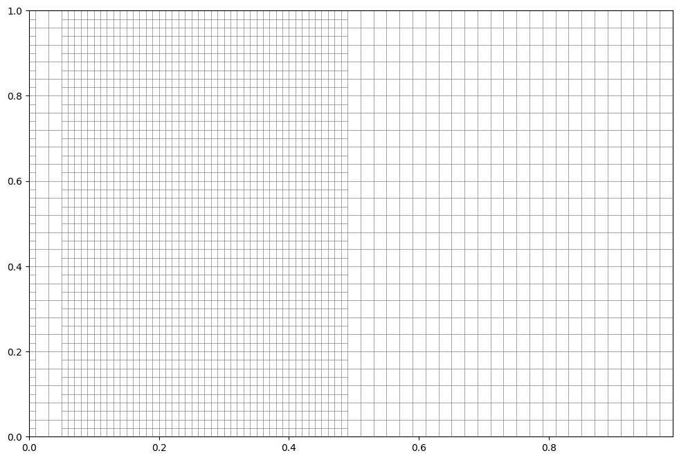
The grid can be visualized via the following method.

[15]:

axis4.plot_grid()

[15]:

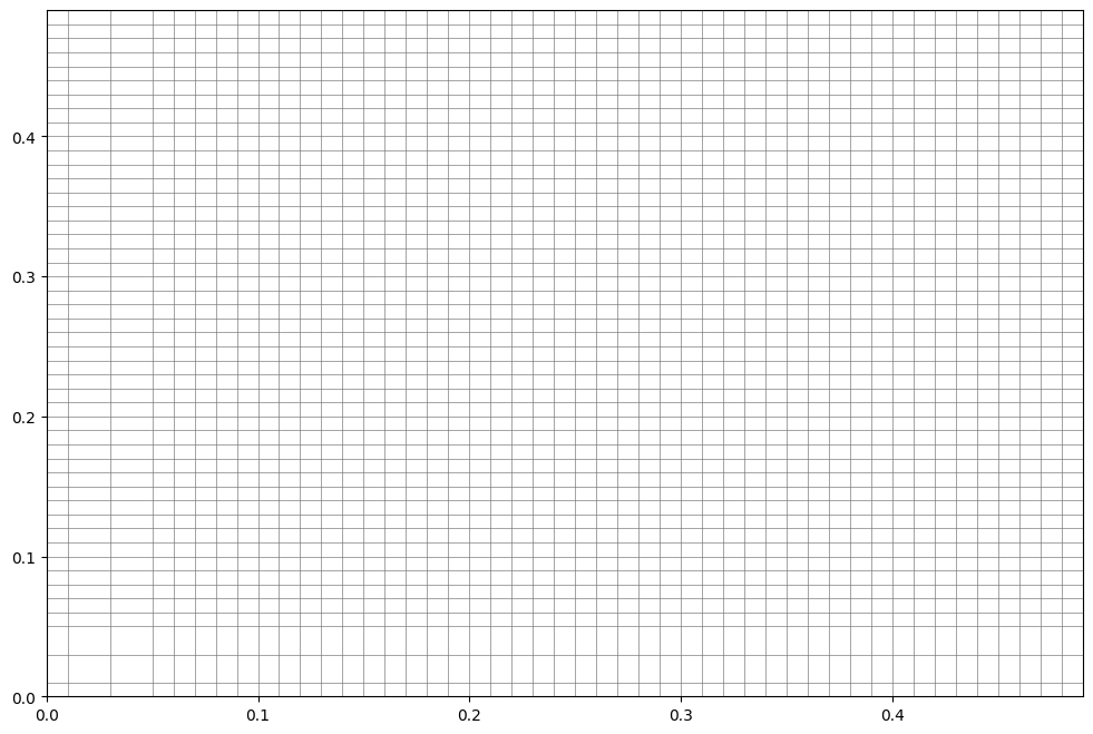
Weighted grid¶

The multiplication of two axis objects expect two objects with different axis_type attributes. It also cerates a grid. In contrast to the addition, the multiplication weights the y-values by the x-values. The weights are currently related to the width of a bin in x-direction.

The following cell uses the merged axis3 from above and the transposed uniformly distributed axis2. It can be seen, that the discretization in z-direction changes with the x-width.

[16]:

axis5 = axis3 * axis2.T
axis5.create_grid()

(1, 73)
(73, 51)

[16]:

<aim2dat.fct.discretization.DiscretizedGrid at 0x7fb94e2db370>

[17]:

axis5.plot_grid()

[17]: